
Quality control not only helps to inspect a product and give an acceptance/rejection decision, but also helps in reducing the number of rejections over time. For this, we need to analyse quality data using statistical methods and get required information on present quality. The information obtained should be used judiciously to improve the quality of a product. In this way, the decisions will not be biased by individual perceptions.
Total Quality Management (TQM) and Six Sigma processes to improve product quality are based on statistical methods. This article discusses some of the statistical methods used in quality control work. Emphasis is given on application and methodology rather than mathematics and related proofs.

The most popular statistical method amongst engineers is sampling technique. Other statistical methods include estimation of limits of a quality parameter with known confidence, statistical control charts, comparing quality parameters of two different lots of units (could be from different vendors), fitting quality data to a theoretical probability distribution function and proportion within specification limits.
Sampling
Sampling is used to accept/reject a large quantity of goods by inspecting a small sample from it. Certain small quantity (as per sampling plan) is selected at random from the goods. Every piece of the sample has to pass or fail a test as per definition given in the test procedure. If failed number of units is less than a defined acceptance number, the entire lot is accepted. Else the entire lot is rejected.
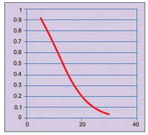
Since acceptance/rejection of the goods is dependent on testing of only a few samples from the lot, risks are involved in this process. Sometimes, a good lot can get rejected and a bad lot can get accepted. The probability of rejecting a good lot is called producer’s risk. The probability of accepting a bad lot is called consumer’s risk. Graph of probability of acceptance versus percentage of defectives in a lot is shown in Fig. 1. It is called operating characteristic.
It can be observed that probability of acceptance decreases as percentage of defectives in a lot increases. Hence a supplier should minimise percentage of defectives in a lot so that the lot could be accepted with high probability. The supplier and consumer should agree on risks acceptable to both of them.
Confidence interval
Many a times, it is necessary to estimate properties of goods from a sample data. For example, if a random sample of 20 capacitors is taken from a large lot of 1000µF bin, and their average is found to be 995 µF, the sample average 995 µF is called point estimate of lot average. This number can be used to estimate population (product)average with certain confidence, which is called confidence interval.
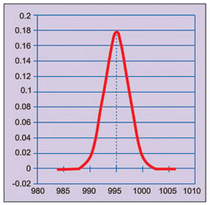
In case the population follows normal distribution, properties of normal distribution can be used to estimate average value of the lot with certain confidence. Graph of normal distribution with population average, say 995 µF, is shown in Fig. 2.
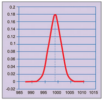
In case the population average is more than 995 µF, say 999 µF, normal distribution would be as shown in Fig. 3. We observe that probability to get observed value of 995 µF or less is very small. So we select an upper limit for population average such that the probability to get observed value or less is small, say 0.025.
In case the population average is less than 995 µF, say 990 µF, normal distribution would be as shown in Fig. 4. Since probability to get the observed value of 995 µF or more is very small, we select a lower limit for population average such that the probability to get observed value or more is small, say 0.025.
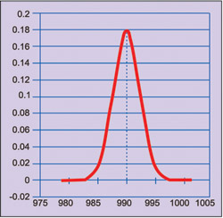
with population average of 990 µF
The gap between lower limit (990 µF) and upper limit (999 µF) is the 95 per cent confidence interval. In other words, the probability of a capacitor’s value being outside these limits is only 5 per cent.
Control charts
Statistical control charts are used to determine whether a manufacturing process is under control or not. There is a random variation in many manufacturing process parameters, which causes output variations. A high number of causes exist, each contributing a small amount of variation to the process output, but none of them dominating. Under these conditions, the output varies within controlled limits. These causes are called common causes. Manufacturing process under such conditions is said to be under statistical control.