Scilab is a FOSS programming environment that aids in numerical computations for engineering and scientific purposes. This tool is used for learning engineering sciences and automatic control engineering. A review of a newer version Scilab 6.0.0 is also available.
Anagha P.
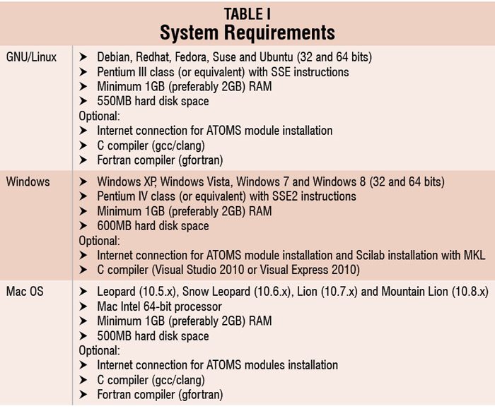
Scilab is a powerful computational workspace and programming language that comes with a rich set of algorithms and other features for various scientific applications. It is a free and open source software (FOSS) project licenced under CeCILL. It is distributed with the source code, and is also available for download in 32- and 64-bit executable versions for GNU/Linux, Windows and Mac OS.
Features
Scilab comes with a large number of functionalities that assist computations. Some of the features of this software are given below:
Mathematics and simulation. Scilab provides 1700 functions that help mathematical operations and data analyses in general science and engineering applications. In addition to the elementary mathematical functions, they can process linear algebra, sparse matrices, polynomials and rational functions. It can also perform various simulations (linear and non-linear differential equation solver).


Optimisation. Scilab provides algorithms to solve constrained and unconstrained continuous and discrete problems for large- and small-scale issues such as optimisations (linear, quadratic, non-linear and linear matrix inequality), semi-definite programming, genetic algorithms and simulated annealing.
Statistics. Data analysis and modelling tools are available for descriptive statistics, probability distributions and linear and non-linear modelling.
Control systems study. Control system design and analysis tools are transfer function, classic and robust control, stability analysis and state-space control system design.
Signal processing. It can perform signal generation, data windowing, power spectral density estimation, analogue filter design, digital FIR and IIR filter design and several signal transforms including Fastest Fourier Transform in the West (FFTW).
Customisation of graphics. There are options provided for 2D and 3D visualisation. You can plot line charts, pie charts and histograms and animate them. These graphics can be saved and exported in PNG, PPM, EMF, EPS, FIG, PDF and SVG formats. The user can also add LaTeX or MathML annotations to it.
Xcos. It is a hybrid, dynamic system modeller and simulator in Scilab. It lets you design, save, load, compile and simulate models of mechanical systems, hydraulic circuits and control systems.
Application development. API enabling is provided to increase the native functionalities. Scilab has tools for creating and deploying user-defined modules. It also allows users to interface with external tools such as Matlab and Excel.
Installation
Source form of Scilab is available, which lets the users compile and produce their own binary format. Binary files for Linux, Windows and Mac OS are also available in 32- and 64-bit platforms. Select the type of file that suits your requirements.
Under Linux. Select the .tar.gz format file for Linux operating system (OS), 32-bit or 64-bit platform depending on the version of your OS. However, if you are not sure whether your OS is 32-bit or 64-bit, it is better to install the 32-bit version binary file. Installation in Linux is simple. Just unzip the file to target directory of your choice. Select the binary executable file Scilab by following the path in target directory scilab-5.x.x > bin > scilab. A script will be executed and then the main window will appear.
Under Windows. Select the suitable binary file for installation. Double click and run this file to open the installation wizard. You can either install the whole package or customise what all libraries need to be installed. For computers with Intel processors, installing Intel Math Kernel Library (MKL) increases the speed of computation.
Under Mac OS. The Mac version binary file for Scilab is in .dmg format. It uses Mac OS installer and follows the classic installation process familiar to Mac users.
Getting started
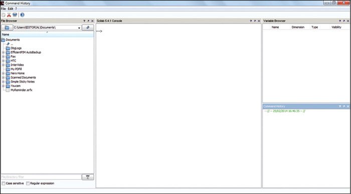
The main window, as shown in Fig. 1, is divided into four sub-sections: the Scilab console in the centre for making calculations, the files browser on the left, the variables browser on the top right and the work history on the bottom left.

In the console window, type any command after the prompt ‘–>’ and press Enter key (in Linux and Windows) or Return key (in Mac OS) from the keyboard to display the result.
Basic numerical calculations
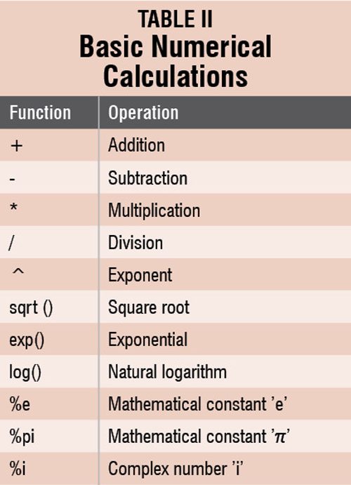
Basic arithmetic operations can be performed in Scilab with simple commands as given in the Table II. It is to be noted that the commands are case-sensitive. For example, only ‘sqrt’ is valid. ‘Sqrt’ and ‘SQRT’ show undefined variable and the calculation will not be performed.
Example. To find the cube, the product of numbers 3 and 5:
–>(3*5)^3
ans =
3375.
First type (3*5)^3 just after the prompt, as in the first line of the script given above. Press Enter/Return. The answer 3375 will be displayed in the console, as in the third line. You can navigate in the console using mouse or the ← ↑ → ↓ arrow keys of the keyboard.
If a semicolon (;) is added at the end of command line, the result would not be displayed in the console window, as given below:
–>(2+4)^2;
Scilab editor
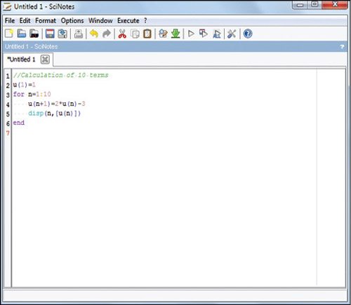
 There are many disadvantages of typing the commands directly in the console window. It is difficult to edit multiple instructions and you cannot save the commands. This is where SciNotes is used. You can launch SciNotes by clicking on the first icon in the toolbar, or go to Applications > SciNotes.
The closing of opened parentheses, end loops, function and test commands are added automatically in the text editor. This can be disabled from menu bar Options > Auto-completion on, and selecting ‘(,[,…’ or ‘if,function,…’ or both. Each instruction is to be entered in a separate line.


