

Want to play around with the acoustic signals or the sound inputs for your audio device? This article guides you on how to start working with VSLM, a tool that allows you to do just that
Sound-level meters are expensive instruments that measure sound or acoustic pressure, and are used to analyse sound signals. Thankfully, there is now a software tool available that allows students to analyse acoustic signals without the need for expensive full-featured sound level meters.

VSLM (Virtual Sound Level Meter) is a program that provides students, educators, researchers and consultants with a tool for analysing calibrated sound level recordings. A user can make calibrated digital recordings of an acoustic signal, and analyse using the software with multiple analysis techniques that allow students to ‘play’ with the analyser and observe what the different settings do to the signals.
VSLM follows the ANSI acoustic measurement and analysis standards, which ensure that the results obtained using VSLM match the results obtained from any other standard measurement equipment. The current version of VSLM implements basic integrating, 1/3 octave band/high-resolution FFT sound level meter functions, noise dose analysis and spectrograms.
The GUI
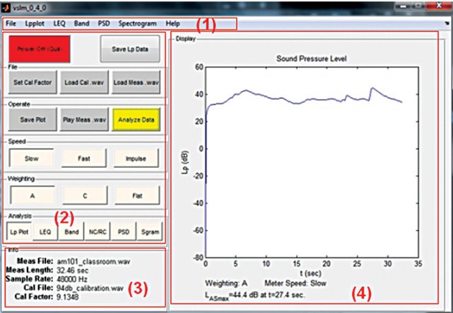
The software’s GUI is made to resemble it with a physical sound analyser. Fig. 1 shows the main GUI. It consists of a main menu (1) at the top for saving and loading various settings. There is a set of analysis buttons (2), which is used for various analysis modes. The info box (3) provides the details of currently selected measurements and calibration. Analysed plots and computed information are displayed in the display area (4).
Calibration
The input .wav files should be calibrated for the analysis. .wav files are generally 16- or 24-bit integers and their inputs need to be converted into Pascals by setting a calibration constant/factor; while for the files that are already calibrated (like some floating point .wav files), the calibration factor should be set to 1.
Integration Time
Note: VSLM’s default calibration factor is 1.
Load Cal .wav. The Load Cal .wav button can be used to load a .wav file that has a calibration recording. After pressing the button, you need to select the calibration recording and enter the calibration level in dB. The rms value of the calibration is then calculated by the system, and the calibration factor is set accordingly. The calibration file name and calibration factor are displayed in the info box (3).
Calibration files are recordings from sound-level calibrators with sound levels of 94, 114 or 124 dB, and the loaded calibrations should be in .wav file format at sample rates of 22.05 kHz, 44.1 kHz, 48 kHz or 96 kHz.
Set Cal factor. If you can estimate the calibration factor for any recording, use this button to manually set the calibration factor. This is particularly useful while performing re-analysis of recordings whose calibration factor is already known, after loading the calibration file.
Manual setting of the calibration factor sets the calibration file name to ‘None Loaded’ while the calibration factor is displayed in info box (3).
Measurement files
The files that are analysed by the system are measurement .wav files.
Load Meas .wav. This button loads the measurement .wav file for analysis. The measurement file must be a standard .wav format audio recording at sample rates of 22.05 kHz, 44.1 kHz, 48 kHz or 96 kHz.
Note: Only the first channel of a multichannel file is analysed and the rest are ignored.
Play Meas .wav (Windows only). This button will play the loaded measurement .wav file via Windows Media Player. This option is available in Windows versions only.
Speed. The speed buttons Slow, Fast and Impulse apply the ANS, S1.4-1983 (R2006) standard exponential time-weighing functions for Lp plot analysis.
Note: Other plot analysis does not apply a time-weighing function.
Slow. This setting applies the ‘Slow’ time response with a time constant = 1.0 seconds. It is the most common setting used in standard sound-level meters, and is best used to estimate the average sound level of sounds with a limited dynamic range, such as speech.
Fast. This setting applies the ‘Fast’ time response with a time constant = 0.125 seconds. It is used for sound levels with a high dynamic range and fairly quick variations in the temporal response.
Impulse. This applies the ‘Impulse’ time response with a time constant = 0.035 seconds for rising signals and 1.5 seconds for falling signals. This function is used to accurately capture peak sound levels of impulsive noises such as gun shots.
Weighting
Weighting buttons A, C and Flat apply the ANSI S1.42-2001 standard weighting or no weighting at all.
A. The A weighting filter is the most often used frequency response filter in acoustic analysis. For low- to-moderate sound levels (under about 80 dB), A-weighted sound levels are a better approximation to perceived loudness than any other weighted sound levels.
C. For higher sound levels (over about 90 dB), C-weighted sound levels are a better approximation to perceived loudness than A-weighted sound levels. If there is significant low-frequency content present in your acoustic signal, C weighting can be used in conjunction with A weighting.
Flat. For no frequency weighting (octave or 1/3-octave band analysis), use Flat weighting.
Analysis
There are three main analysis modes: time domain, frequency domain and mixed domain. Time domain analysis includes Lp mode and LEQ mode; frequency domain analysis includes Band mode and PSD mode; and mixed domain analysis is the Sgram or spectrogram mode.
Select the analysis mode by pressing the ‘Analysis’ button of any of the above modes and then press the yellow ‘Analyse Data’ button.
Note: If there is no measurement file loaded, a warning is displayed.
Lp Mode
Select Lp mode to get the analysis of a standard non-integrating sound level meter.
Settings.
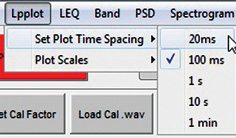
1. Select Lpplot→Set Plot Time Spacing from the main menu (1) [Fig. 2], to select the sample rate of the signal stimulated in Lp mode.
2. Select Lpplot→Plot Scales from the main menu (1) [Fig. 2], to select the plot scales as auto for auto scaling, or as manual for manually setting the X and Y minimum and maximum values.
LEQ Mode
Select LEQ mode to get the analysis of a standard integrating sound level meter. LEQ takes a measurement file to compute a series of 100ms LEQs applying the selected frequency weighting.
Settings.
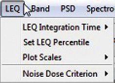
1. Select LEQ→LEQ Integration Time from the main menu (1) [Fig. 3], to set the length of the LEQ integrations, which are plotted and saved.
2. Select LEQ→Set LEQ Percentile from the main menu (1) [Fig. 3] to enter a level of percentile for computation and display.
3. Select LEQ→Plot Scales from the main menu (1) [Fig. 3], to select the plot scale as auto for auto scaling, or as manual for manually setting the X and Y minimum and maximum values.
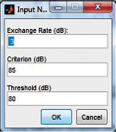
4. Select LEQ→Noise Dose Criterion from the main menu (1) [Fig. 3], to open a dialogue box [Fig. 4] and enter the Exchange rate, Criterion and Threshold values.
Band Mode
Select Band mode to compute the overall LEQ in the octave or 1/3 octave bands.
Settings.
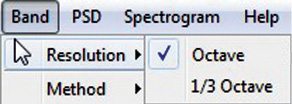
1. Select Band→Resolution from the main menu (1) [Fig. 5], to select the resolution from octave or 1/3 octave.
2. Select Band→Method from the main menu (1) [Fig. 5], to select the method FFT or ANSI.
NC/RC Mode
Select this mode to compute Noise Criterion (NC) and Room Criterion (RC) Mark II ratings for the octave band, unweighted, LEQ spectrum of the measurement file.
Settings.
There are no user settings available for this mode.
PSD Mode
PSD mode analyses the overall power spectral density using a variation of the Welch Modified Periodogram method.
Settings.
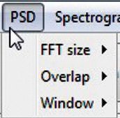
1. Select PSD→FFT Size from the main menu (1) [Fig. 6], to select the FFT size from the 256, 512, 1024, 2048, 4096 or 8192 pt FFT options.
2. Select PSD→Overlap from the main menu (1) [Fig. 6], to select the overlap percentage.
3. Select PSD→Window from the main menu (1) [Fig. 6], to select the FFT window type (Hanning, Hamming or Flat Top).
Sgram Mode
The Sgram button breaks the measurement file into small segments of a selectable size and computes the Welch Modified Periodogram method for each segment.
Settings.
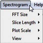
1. Select Spectrogram→ FFT Size from the main menu (1)
[Fig. 7], to select the FFT size from the 256, 512, 1024, 2048, or 4096 pt FFT options (default is 512).
2. Select Spectrogram→Slice Length from the main menu (1) [Fig. 7], to select the size of the buffer for each segment from the options of 100ms, 1s and 10s.
3. Select Spectrogram→Plot Scale from the main menu (1) [Fig. 7], to set the maximum dynamic range in each plot. The software truncates all data above 30 dB and 50 dB when 30 dB and 50 dB are selected, respectively. Selecting Auto will let the software choose the plot scale.
4. Select Spectrogram→View from the main menu (1) [Fig. 7], to display the resulting time-frequency plot (as 2D or 3D plots).
Save Analysis. This button saves the most recent analysis to a text file.
Different data are saved for different analysis modes:
1. For Lp plot mode, the time and Lp are saved.
2. For LEQ mode, the time and LEQ are saved. The header will include Ln statistics and Noise Dose information (if applicable).
3. For Band mode, the centre frequencies and Band LEQ are saved.
4. For NC/RC mode, the NC/RC levels and octave band LEQ are saved.
5. For PSD mode, the frequency and power spectral density are saved.
6. Sgram mode has too much data to be saved in a text file, so the display figure is copied as a MATLAB figure and figure export function is called.
Save Plot
This button copies the current display figure as a MATLAB figure, and then the export function is called, which can be used to alter the size and font of the figure and then save it.
If you have been looking for a sound level meter to analyse the sound output from your audio device, this tool is for you. You can use it to play around with a calibrated sound recording, and implement different analysis techniques and observe their effect on the signals. Have fun!
Pankaj V. is a technical journalist at EFY Gurgaon