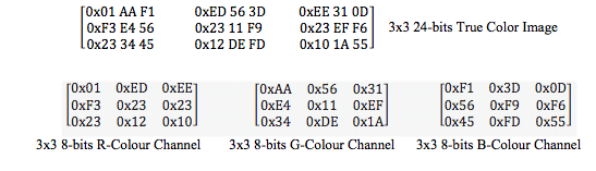
The images in JPEG format are true colour images with 24-bit colour resolution. A 24-bit colour image is the combination of R-, G- and B-colors (8-bits each) ranged from 0 to 255, where 0 being the perfect black and 255 is the complete red, green and blue respectively in each colour domain. 8-bits R-, G- and B-color channel value are concatenated to form 24-bit RGB colour value in jpeg image format. This can be explained in the following way:
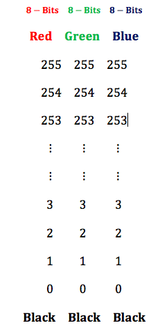
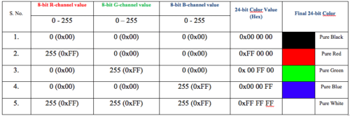
From above, it can be observed that there are 256 x 256 x 256 = 224 = 1,67,77,216 no. of combinations (colors) possible using different R-, G- and B-color channel values. Being 8-bit in each colour channel, the final colour is 24-bit in colour resolution. Table-1 shows the pure colours along with 24-bit hex value using extreme values in each colour channel.
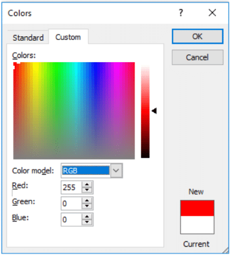
Further, more colours can be reproduced using different combinations of colour channel values. This can be exercised in colour palette available in any MS office tool (MS Paint).
JPEG image may, therefore, be split into R-, G- and B-color channels in order to view the histogram in individual colour channels.

Histogram – is the plot between no. of pixels Vs pixel intensity. For example, in the below-given pixel image of 4×4 size, figure 2(b), followings are the statistics:
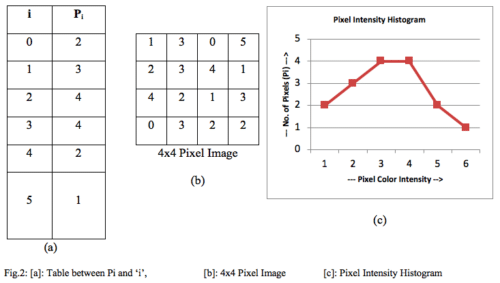
Where Pi is no. of pixels of color intensity 0 to 5 here ‘i’, figure 2(a). The Pixel intensity histogram of the same is given in the right end of the above figure-2 (c).
R-, G- and B-Color Histogram
JPEG images are true color images and have 24-bits color resolution. When a JPEG format image is read in MATLAB environment using the command imread(), the image is read in three colour channel matrices namely R-, G- and B-color channel. This can be understood in below 3×3 example.
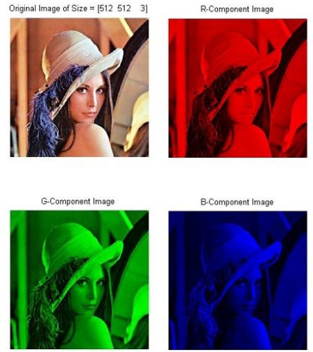
Individually, the R-, G- and B- colour channels are 8-bit in resolution; however, to view the image into different colour channels, the R-, G- and B- colour channels are converted back to 24-bit colour channel by making remaining colour channels as black (Blank Image). This is explained below: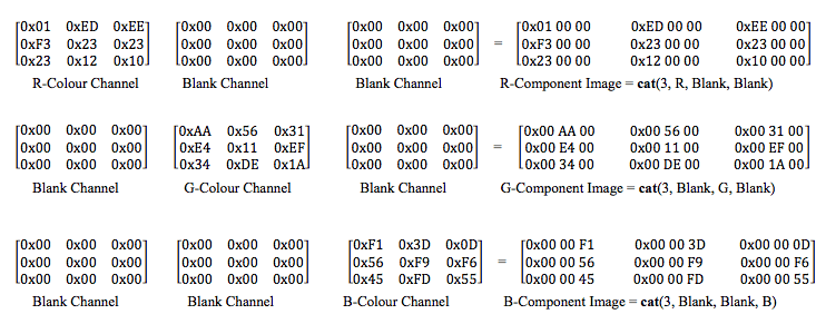
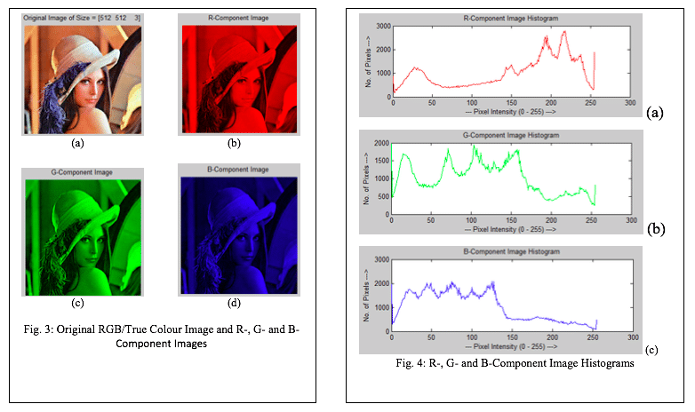
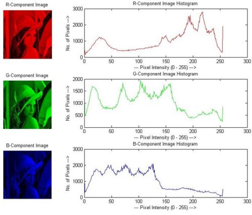
Therefore, each colour channel has its own histogram and the true colour image can be viewed into different colour channels separately, figure-3(a, b, c and d). The R-, G- and B-colour histograms of the same image are also shown in figure 4(a), (b) and (c) respectively.
- The command imhist() is used in matlab to compute the histogram of an input image. The code given here computes the histogram in different color channels of the image.
- cat command concatenates the matrix arrays R-, G- and B- color channels along with Blank image to give R-, G- and B-color component image view.
The working code for R-, G- and B- Histogram Extraction using Matlab is given in below text box.
Code for R-, G- and B- Histogram Extraction
***** Code Starts here *****
close all,
clear all,
clc,
ProjectPath = pwd;
ImagePath = strcat(ProjectPath,’\Leena.jpg’);
PlotRow = 2;
PlotCol = 2;
Orig = imread(ImagePath);
subplot(PlotRow,PlotCol,1); imshow(Orig);
[row col c] = size(Orig);
str = strcat(‘Original Image of Size = [‘,num2str(size(Orig)),’]’);
title(str);
Blank = zeros(row,col);
R = Orig(:, :, 1);
R_Comp_Image = cat(3,R,Blank,Blank);
subplot(PlotRow,PlotCol,2); imshow(R_Comp_Image);
title(‘R-Component Image’);
G = Orig(:, :, 2);
G_Comp_Image = cat(3,Blank,G,Blank);
subplot(PlotRow,PlotCol,3); imshow(G_Comp_Image);
title(‘G-Component Image’);
B = Orig(:, :, 3);
B_Comp_Image = cat(3,Blank,Blank,B);
subplot(PlotRow,PlotCol,4); imshow(B_Comp_Image);
title(‘B-Component Image’);
PlotRow = 3;
PlotCol = 2;
figure,
subplot(PlotRow,PlotCol,1); imshow(R_Comp_Image);
title(‘R-Component Image’);
subplot(PlotRow,PlotCol,2);
[P,X] = imhist(R); plot(X,P,’r’);
title(‘R-Component Image Histogram’);
xlabel(‘— Pixel Intensity (0 – 255) —>’);
ylabel(‘No. of Pixels —>’);
subplot(PlotRow,PlotCol,3); imshow(G_Comp_Image);
title(‘G-Component Image’);
subplot(PlotRow,PlotCol,4);
[P,X] = imhist(G); plot(X,P,’g’);
title(‘G-Component Image Histogram’);
xlabel(‘— Pixel Intensity (0 – 255) —>’);
ylabel(‘No. of Pixels —>’);
subplot(PlotRow,PlotCol,5); imshow(R_Comp_Image);
title(‘B-Component Image’);
subplot(PlotRow,PlotCol,6);
[P,X] = imhist(B); plot(X,P,’b’);
title(‘B-Component Image Histogram’);
xlabel(‘— Pixel Intensity (0 – 255) —>’);
ylabel(‘No. of Pixels —>’);
***** End of Code *****