Artificial Neural Network Simulation in Labview and Matlab

Artificial neural network, in essence, is an attempt to simulate the brain. When the user enters the inputs (say, p1, p2 and p3) and the expected corresponding outputs (say, t1, t2 and t3) in the program, the program trains the system and gives a final weight. The final weight is computed to get the final expected output. This program is an attempt to understand the basics of artificial neural network and how one can use it for further applications.

Artificial neural network
Artificiawhen a gender recognition net is presented with a picture of a man or woman at its input node, it must set an output node to 0.0 if the picture depicts a man or to 1.0 for a woman. In this way, the network communicates its knowledge to the outside world.l neural network theory revolves around the idea that certain key properties of biological neurons can be extracted and applied to simulations, thus creating a simulated (and very much simplified) brain. The first important thing to understand is that the components of an artificial neural network are an attempt to recreate the computing potential of the brain. The second important thing to understand, however, is that no one has ever claimed to simulate anything as complex as an actual brain. Whereas the human brain is estimated to have of the order of ten to a hundred billion neurons, a typical artificial neural network is not likely to have more than a thousand artificial neurons.

In theory, an artificial neuron (often called a ‘node’) captures all the important elements of a biological one. Nodes are connected to each other and the strength of these connections is normally given by a numeric value between -1.0 (for maximum inhibition) and +1.0 (for maximum excitation). All values between the two are acceptable, with higher-magnitude values indicating a stronger connection strength. The transfer function in artificial neurons, whether in a computer simulation or actual microchips wired together, is typically built right into the node’s design.

- Advertisement -

A transfer function (also known as the network function) is a mathematical representation, in terms of spatial or temporal frequency, of the relationship between the input and output of a linear time-invariant system.

Perhaps the most significant difference between artificial and biological neural nets is their organisation. While many types of artificial neural nets exist, most are organised according to the same basic structure. There are three components to this organisation: a set of input nodes, one or more layers of ‘hidden’ nodes, and a set of output nodes. The input nodes accept information, and are akin to sensory organs. Whether the information is in the form of a digitised picture, a series of stock values or just about any other form that can be numerically expressed, this is where the net gets its initial data. The information is supplied as activation values, that is, each node is given a number, with higher numbers representing greater activation.

- Advertisement -

This is just like human neurons, except that rather than conveying their activation level by firing more frequently—as biological neurons do—artificial neurons indicate activation by passing this activation value to connected nodes. After receiving this initial activation, the information is passed through the network. Connection strengths, inhibition/excitation conditions and transfer functions determine how much of the activation value is passed on to the next node.

Each node sums the activation values it receives, arrives at its own activation value, and then passes that along to the next nodes in the network (after modifying its activation level according to its transfer function). Thus the activation flows through the net in one direction—from input nodes, through the hidden layers, until eventually the output nodes are activated.

If a network is properly trained, this output should reflect the input in some meaningful way. For instance, when a gender recognition net is presented with a picture of a man or woman at its input node, it must set an output node to 0.0 if the picture depicts a man or to 1.0 for a woman. In this way, the network communicates its knowledge to the outside world.

How they learn
Having explained that connection strengths are storehouses of knowledge in neural net architectures, it should come as no surprise that learning in neural nets is primarily a process of adjusting connection strengths. In neural nets of the type described so far, the most popular method of learning is called ‘perceptron,’ which is a basic algorithm to learn neural network theory.

The perceptron is a type of artificial neural network invented in 1957 at the Cornell Aeronautical Laboratory by Frank Rosenblatt. It can be seen as the simplest kind of feedforward neural network: a linear classifier. The perceptron is a binary classifier which maps its input ‘x’ (a real-valued vector) to an output value ‘f(x)’ (a single binary value):

where ‘w’ is a vector of real-valued weights, ‘w.x’ dot product (which here computes a weighted sum) and ‘b’ bias (a constant term that does not depend on any input value).

The value of ‘f(x)’ (0 or 1) is used to classify ‘x’ as either a positive or a negative instance, in the case of a binary classification. If ‘b’ is negative, the weighted combination of inputs must produce a positive value greater than |b| in order to push the classifier neuron over the ‘0’ threshold. Spatially, the bias alters the position of the decision boundary. The perceptron learning algorithm does not terminate if the learning set is not linearly separable.

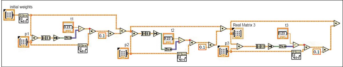
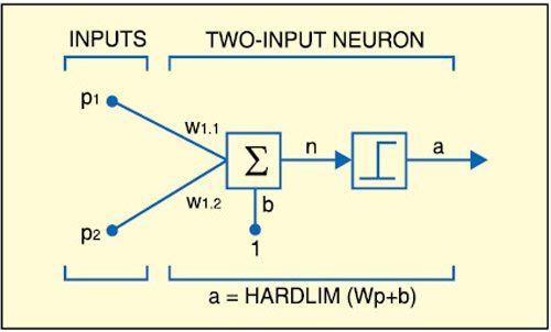
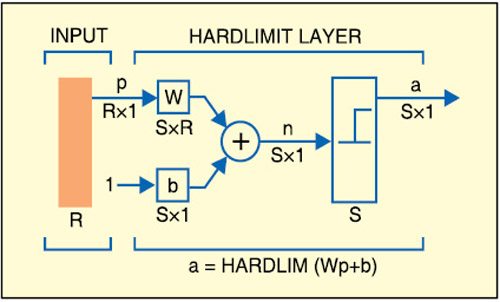
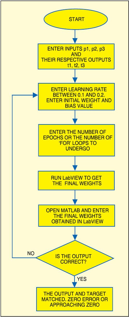
In Fig. 1, p1 and p2 are the inputs to the system. These are implemented in LabVIEW. The inputs are then weighted with some suitable values such as w1,1 and w1,2. Now the inputs ‘p’ and ‘w’ are multiplied and all the products (p×w) are added. Since the values obtained after this step are random real numbers, they need to be converted into a binary number. This is obtained by using the hardlimit functions (refer Fig. 2) like unit step or signum function. After a number of iterations, the final weights are obtained.

In Figs 1 and 2, ‘b’ represents bias, ‘n’ number of types of inputs, ‘R’ real number, and ‘S’ unit step function to convert the real number into 1’s and 0’s. Rx1 and Sx1 represent multiplication.
The final weights are computed to get the final output using MATLAB.

LabVIEW block description

LabVIEW is a graphical programming environment that allows you to design and analyse a digital processing system in a shorter time than text-based programming environments. LabVIEW graphical programs are called virtual instruments.

Virtual instruments run based on the concept of data flow programming. This means that execution of a block or a graphical component is dependent on the flow of data, or more specifically a block executes when data is available at all of its inputs. Output data of this block is then sent to all other connected blocks.

A virtual instrument consists of two major components: a front panel and a block diagram. The front panel provides the user-interface of a program, while the block diagram incorporates its graphical code. The block diagram contains terminal icons, nodes, wires and structures. Terminal icons are interfaces through which data is exchanged between a front panel and a block diagram. A virtual instrument is designed by going back and forth between the front panel and the block diagram, placing inputs/outputs on the front panel and building blocks on the block diagram.

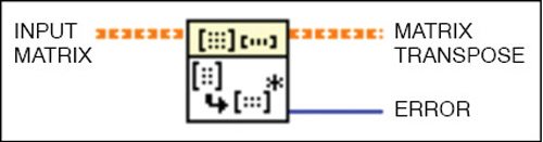
In this artificial neural network, the block diagram includes real transpose matrix, nodes, wires, structures, etc.

Real transpose matrix is used to transpose the matrix having real number.

The input matrix is fed to the block and the output matrix transpose is obtained in the orange line. Errors, if any, can be observed in blue line (refer Fig. 4).

The matrix transpose output is fed to another block, which converts the real matrix from 3D into 2D array for further processing.

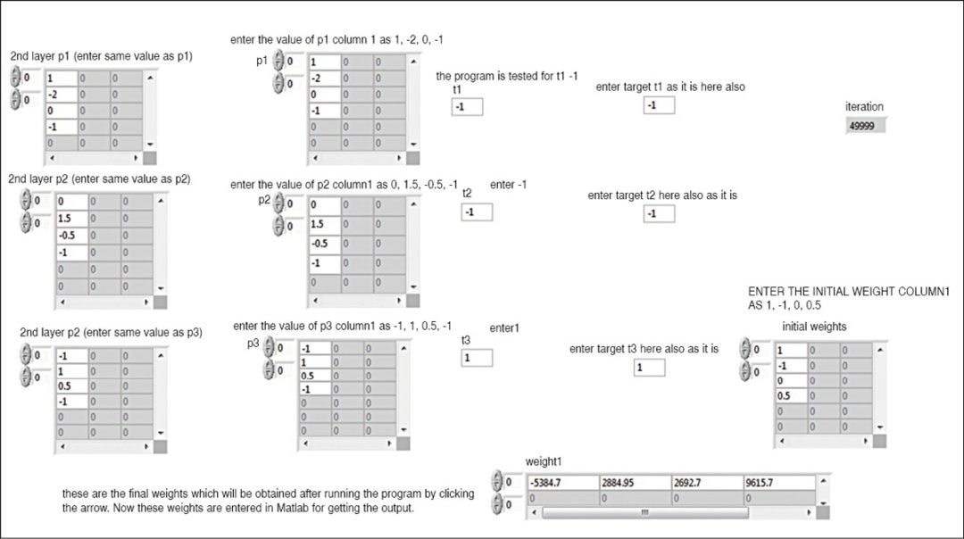
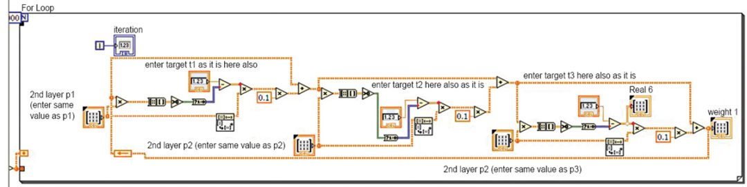
The feeding of inputs and initialisation of weights are done in the first stage of the block (Fig. 5). That is, the first iteration is done in this stage. The entire calculation and weight inputs from the first stage are now fed to the second stage (Fig. 6) for further processing to train the system. The iterations are completed and the final weights obtained in the second stage.

Learning algorithm
Here we explain learning algorithm for a single-layer perceptron. For multilayer perceptrons, more complicated algorithms such as backpropagation must be used. Alternatively, methods such as the delta rule can be used if the function is non-linear and differentiable, although the one below will work as well.

The learning algorithm we demonstrate is the same across all the output neurons. Therefore everything that follows is applied to a single neuron.

We first define some variables:

y = f(Z) denotes the output from the perceptron for input vector ‘Z’

‘b’ = Bias, which in the example below is taken as 0

D = {(x1, d1), …, (xs, ds)} is the training set of ‘s’ samples, where ‘xj’ is the n-dimensional input vector and ‘dj’ is the desired output value of the perceptron for that input.

We show the values of the nodes as follows:

xj, i = Value of the ith node of the jth training input vector

xj, 0 = 1

Weights are represented by wi, which is the ith value in the weight vector, to be multiplied by the value of the ith input node.

An extra dimension, with index n+1, can be added to all input vectors, with xj, n+1 = 1, in which case wn+1 replaces the bias term. To show the time-dependence of ‘w’, we use wi(t), which is weight i at time t.

α = Learning rate, where 0<α≤1

Too high a learning rate makes the perceptron periodically oscillate around the solution unless additional steps are taken.

Appropriate weights are applied to the inputs, and the resulting weighted sum is passed to a function that produces the output ‘y’.