Artificial Neural Network Simulation in Labview and Matlab

Learning algorithm steps. With the variables defined above, we will calculate the output as follows:

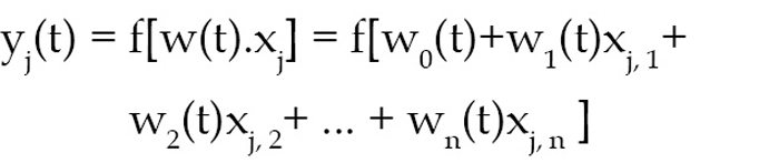
First, calculate the actual output using the function:

- Advertisement -

Second, adapt weights as follows:
wi(t+1) = wi(t)+α(dj–yj(t))xj,i for all nodes 0≤i≤n.

Now proceed as follows:
1. Initialise weights w1, w2, w3, w4 and threshold, which has been done internally in the program. Note that weights may be initialised by setting each weight node wi(0) to ‘0’ or a small random value.

- Advertisement -

2. For each sample ‘j’ in our training set ‘D’, perform the following steps over the input xj (in the LabVIEW program, inputs are p1, p2, p3 and p4) and desired output dj (in the program it is t1, t2, t3 and t4).

3. The weights are updated after the program is simulated for 5000 iterations and a final weight is obtained, which gives a proper set of equation for operation.

Step 2 is repeated until iteration error dj–yj(t) is less than user-specified error threshold γ, or a predetermined number of iterations have been completed. This error is calculated by subtracting the output obtained through an iteration from the desired output. This has to be done in both stages of LabVIEW as adder and subtractor blocks (refer Figs 5 and 6).

In the LabVIEW program (Fig. 3), there are two stages which are responsible for training the system and making the system learn. First of all, the user enters the value. This value is fed to stage one, which completes one iteration and performs all the tasks as explained above. Now the output of the first stage and its updated weight becomes the input of the second stage along with the user inputs p1, p2, p3 and p4, and thus remaining 4999 iterations are performed.

It should be noted that a proper selection of the number of iterations is required in order to get the correct output. After proving the weights, inputs and threshold, the LabVIEW is simulated by clicking ‘arrow’ button. After 5000 iterations, the final weights are updated.

With inputs p1, p2 and p3 fed into LabVIEW, you will get final weights (w) as -5384.2, 2884.4, 2692.95 and 9615. The complete flow-chart of the program is shown in Fig. 7.

4. The final weights are fed to MATLAB program to get the desired output. Here you get the output as h = -1

The program has been developed with the condition that for a group of inputs its output is -1. You may use 1 or 0 but in that case you need to change the initial conditions and number of iterations. You can have an output other than this number. for example, when you give the input as orange, apple and grape, the output can be orange, red and green.

Download source code: click here

Testing steps
1. Install LabVIEW evaluation version and MATLAB 10.0 in your system. LabVIEW can be downloaded from National Instruments’ website.

2. Launch LabVIEW from the desktop.

3. Select Blank IV option and open the LabVIEW program (Perp.vi).

4. Enter the inputs between 2 and –2. All dimensions should be 4×1 matrix. Make sure that you do not even touch any data entry point other than the four points of the column in the LabVIEW front panel. The matrix dimensions have to be matched. If you click the input point, its colour will change to white, which will make the size of matrix as 5. Hence data size will be incompatible.

5. Enter learning rate of 0.1 to 0.2. Click arrow (→) on the menu bar to run the program.

6. The final weights will be obtained right below the screen. Enter these values in MATLAB code (perceptronopbipolar.m) and run the program to get the desired output h = -1.

The author is a BE in electronics & telecommunication. His interests include MATLAB, LabVIEW, communication and embedded systems