3. Download the source code from http://sourceforge.net/projects/opencvlibrary/files/opencv-unix/2.3/. It is recommended that you move the downloaded OpenCV package to your /home/ directory. With that as your current directory, extract the archive, as follows:
[stextbox id=”grey”]$ tar -xvf OpenCV-2.3.1a.tar.bz2
cd OpenCV-2.3.1/[/stextbox]
4. Make a new directory called ‘build’ and change directory into it (that is, mkdir build; cd build).
5. Run Cmake as given below:
[stextbox id=”grey”]$ cmake -D WITH_TBB=ON -D BUILD_NEW_
PYTHON_SUPPORT=ON -D WITH_V4L=OFF-D
INSTALL_C_EXAMPLES=ON -D INSTALL_
PYTHON_EXAMPLES=ON -D BUILD_
EXAMPLES=ON ..[/stextbox]
6. Follow this with ‘make’ and ‘sudo make install’ (to install the library).
7. Next, configure the system to use the new OpenCV shared libraries. Edit a configuration file with sudo gedit /etc/ld.so.conf.d/opencv.conf. Add the following line at the end of the file (it may be an empty file, which is okay) and then save it:
[stextbox id=”grey”]/usr/local/lib[/stextbox]
Close the file and run sudo ldconfig.
8. Open your system bashrc file (for me, that is sudo gedit /etc/bash.bashrc) and add the following code at the end of the file:
[stextbox id=”grey”]PKG_CONFIG_PATH=$PKG_CONFIG_PATH:
/usr/local/lib/pkgconfig
export PKG_CONFIG_PATH[/stextbox]
9. Save and close the file, then log out and log in again, or reboot the system.


Examples of image processing
Now let us see how to use the OpenCV library via the Python interface to perform image processing-based tasks.
Here is an explanation of OpenCV syntax and how to use it, along with a few examples. We need not go into the basics of Python code and syntax since that is extensively documented; see http://www.python.org/doc/ for more.
Reading and displaying an image. Our first example named ‘test.py’ is written in Python (refer EFY Note about the source code of this article).
Open the terminal, navigate to the directory that contains the test.py file and run it with ‘python test.py’ command. Here, 12.png is the name of the image file stored under home/jayneil/ folder. You can change the name of the folder if you wish, but you will have to change it in the source code too. The output is as shown in Fig. 2.
The functions in test.py code can be explained as given below.
The ‘Import’ function imports the OpenCV module ‘cv’ so that you can use it, then call the ‘LoadImage’ function (passing the full path to the file, which is needed) to load the image into the variable src.
The ‘NamedWindow’ function creates a window to display the loaded image. The first parameter is the name for the window, and the second sets the sizing mode to automatically resize the window to the size of the image.
‘ShowImage’ is used to display the image in the window, passing it the name of the window and the image variable.
‘WaitKey’ is used so that you can see the image for a sizeable period of time (similar to a delay function).
Finally, ‘DestroyWindow’ destroys the window and frees the resources it used.
Converting an RGB image to gray scale format. Most digital images use the RGB colour model, in which every pixel has three components—red, green and blue. By varying the amount of each component, a pixel gets a unique colour.
Grayscale is another popular colour model, with only one component that varies from 0-255; 0 represents black, and 255 white (for an 8-bit image). The rgb2gray.py code converts an image from RGB to gray scale, which is essential for image detection.
Running this code will give output as shown in Fig. 3. In the eighth line, we have created our own image, similar to the source image (src). The ‘GetSize’ returns the properties of the source image—so our new image has the same dimensions as the source. ‘CreateImage’ takes three parameters: the image dimensions, the colour depth of the image (8-bit or 16-bit) and the number of channels (which, for gray scale, is one). We used the ‘CvtColor’ function to convert the image to gray scale. This function has three parameters. The first one is the source image which we want to convert and the second denotes the destination variable. The third parameter performs the type of conversion desired. In this case it is from RGB to gray scale.
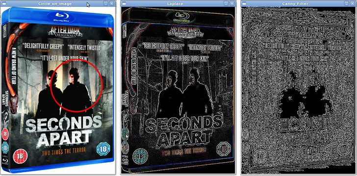
Drawing a circle on an image. You can also edit or manipulate a given image, for example, by drawing a circle in or around it. The circle.py code does this.
After running the code you will get output as shown in Fig. 4. From the ninth to the 11th line in circle.py code, we have described the parameters of the circle—its thickness, line type and co-ordinates. In line 12, the ‘circle’ function is used, which has six parameters: the target image on which to draw the circle, the coordinates, the radius of the circle, the colour of the circle, the thickness and the line type.
The Laplacian of an image. Often, the Laplace operation is performed on an image to get the edges. The laplace.py code does this.
Fig. 5 shows the output of the code given above. The ‘print’ function outputs the properties of the image. In the 10th line of laplace.py code, the Laplace function is used to obtain the edges. It takes two parameters—the source image and the variable in which to store the processed image. You can use ‘SaveImage’ to save the resultant image, supplying the path, the file-name and the variable containing the image. Then load the saved image and display it.
The Canny filter. This is a very popular filter, which is used to very accurately detect the edges in an image. The canny.py code does this.
Run the canny.py code and you will get output as shown in Fig. 6. Convert the input image to gray scale first (see the ninth line), before applying the Canny filter in the 15th line. This function takes five parameters: the source image, the variable in which to store the processed image, and the rest are the threshold values for this filter.
Face detection
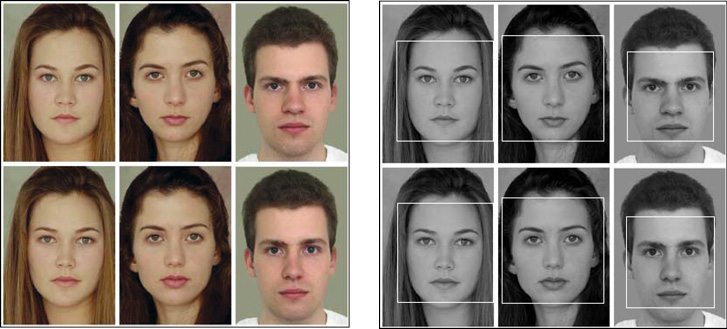
Now, let us detect faces from still images (refer Fig. 7) using a Haar classifier. The Haar classifier is a pre-made program, which you can train to do operations based on your needs. The more you run the program, the more the Haar classifier learns and trains itself. All Haar classifiers are located in OpenCV-2.3.0/data/haarcascades. The face.py code does this.

Run the face.py code and the output is as shown in Fig. 8. In the ninth line of face.py code the Haar classifier is stored which you may use in a variable, as given below:

[stextbox id=”grey”]hc=cv.Load(“/home/jayneil/
haarcascade_frontalface_
default.xml”)[/stextbox]


