This utility program can be a handy tool for anyone working in the field of signal processing with interest in implementation of the project through C++ programming. Although this work can be easily implemented in Matlab using simple inbuilt functions, the real challenge of designing and understanding the concept of filter design will be missed out. In order to understand the depth of designing an FIR filter using window functions, coding in C++ is a must. Described here is a C++ implementation of finite impulse response (FIR) filters using Blackman window method.
FIR filters
The term filter is often used to denote systems that process the input in a specified way. In this context, filtering describes a signal-processing operation that allows signal enhancement, noise reduction or increased signal-to-noise ratio. Systems for the processing of discrete time signals are also called digital filters. Depending on the requirement and application, the analysis of a digital filter may be carried out in time domain, z-domain or frequency domain.
A common application of digital filters is to modify the frequency response is some specified way. An ideal low-pass filter is one of the common examples of digital filters which passes the frequencies up to a specified value and blocks other frequencies. One way to approximate the ideal low-pass response is to do truncation of the impulse response by multiplication with the window functions. Mathematically, it can be expressed as follows:

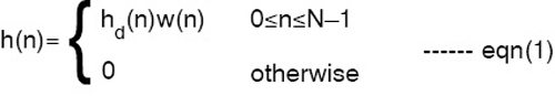
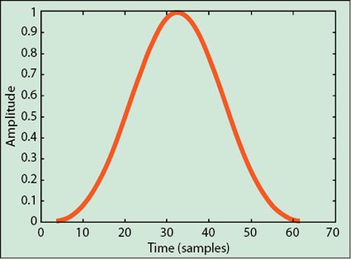
where hd(n) is an infinite-duration impulse response and w(n) is the window function. There are various windows available in signal processing literature. However, in this article we specifically discuss Blackman window. In the case of Blackman window, w(n) is given as:
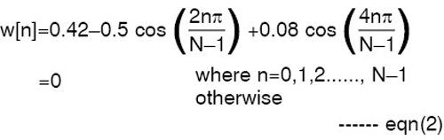
Plot of eqn(2) can be seen graphically as shown in Fig. 1.
Software design
Here, we have developed C++ based software for designing FIR filters using Blackman window to get frequency response. The resultant software has the following salient features:
1. Welcome screen of Blackman window design
2. It prompts you to enter filter’s type
3. It prompts you to enter window length (N) from 1 to 200
4. It prompts you to enter the cutoff frequency. The software is designed to accept the values in radians between 0.2 and 2.6
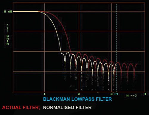
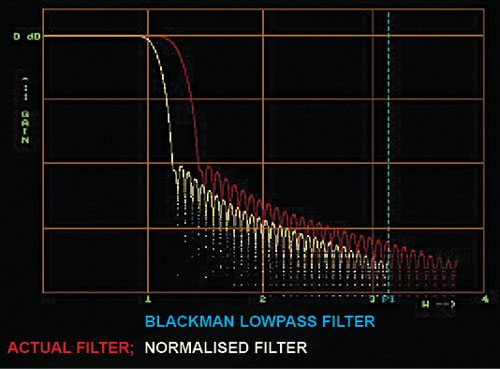
5. The program outputs normalised filter response. This is a filter response which is designed to pass through a cutoff frequency of 1 radian
6. The program outputs actual filter response. This is a filter response which is designed to pass through a cutoff frequency specified by the user
Software structure
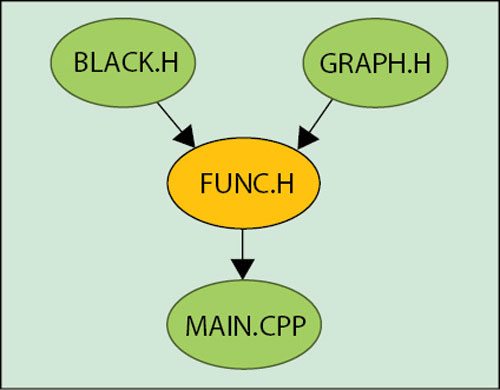
The software is designed to follow the structure as shown in Fig. 2, where the details of each file are explained as given below.
1. MAIN.CPP. This file contains the menu-driven program for user inputs
2. FUNC.H. It is a header file containing code related to Blackman window coefficients calculation
3. BLACK.H. It is a header file containing code for supporting C++ graphics
4. GRAPH.H. It is a header file again to support graphic content in C++
Output responses of the filter
Now, the results obtained after running the software is presented for Blackman window for a low-pass FIR filter for different window length N to observe the effect of N on frequency response. All values of |H(jω)| are in decibels. A normalised frequency scale is used.
Low-pass filter. Simulation of low-pass filter using Blackman window is done through the software. Figs 3 to 5 are the outputs of the low-pass filter for different window length of N=49, 99 and 149, respectively.
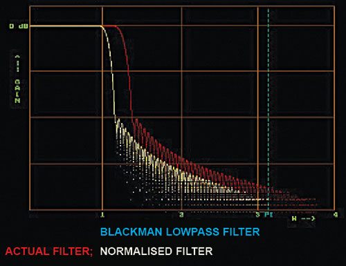
From Figs 3 to 5, we have following observations when N increases from 49 to 149 at cutoff frequency (fc)=1.2:
1. The widths of the pass band and side lobes decrease
2. The slope of the transition band increases, that is, the band develops a sharper cutoff
3. As N increases, the number of ripples increase in the pass band
4. The amplitude and shape of the end-ripple remains the same but it gets shifted towards the edge and finally out of the pass band for larger values of N
5. As N increases, the ripples in the pass band get smoothed out. A key difference in the observed responses of the rectangular is the absence of the Gibbs phenomenon. This owes itself to the smoother shape of the Blackman window in the time-domain, with the notable absence of a discontinuity that would lead to the Gibbs phenomenon.
6. As N increases the widths of the lobes decrease in the stop band
Other frequencies
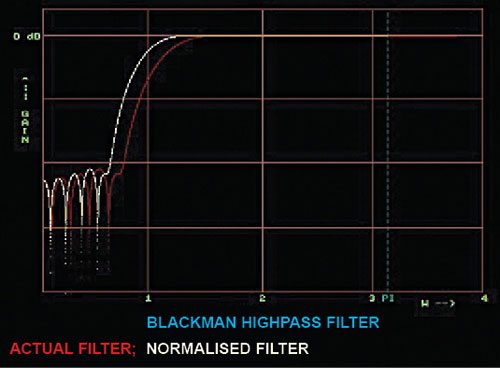
In the next section we present the outputs of high-pass, band-reject and band-pass filters.
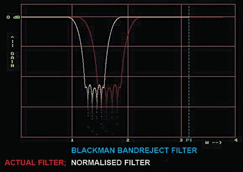
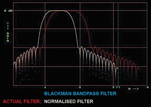
Frequency response of high-pass filter with N=45, fc=1.2 is shown in Fig. 6. Frequency response of band-reject filter with N=67, with lower cutoff frequency (fl)=1.2 and upper cutoff frequency (fu)=2.0, is shown in Fig. 7. Frequency response of band-pass filter with N=91, fl=1.2 and fu=2.0 is shown in Fig. 8.