Image Compression Using Discrete Cosine Transform Technique

Presented here is a MATLAB-based program for image compression using discrete cosine transform technique. It works for both coloured and grayscale images.

Over the last few years, messaging apps like WhatsApp, Viber and Skype have become increasingly popular. These applications let users send and receive text messages and videos. All of us make extensive use of these applications without knowing what actually goes behind the scene in transmitting high-quality images and text. This article dwells on the image/video compression concept that is being used by nearly all the Internet-based messaging applications.

Fig. 1 shows screenshots of the author’s mobile as it compresses the video using WhatsApp software. The application performs compression in two steps: (a) preparing mode and (b) sending mode. The sending mode basically deals with transmission of data stream onto the communication channel. So here we will restrict ourselves to discussing the typical image/video compression algorithm that runs behind the preparing mode.

- Advertisement -

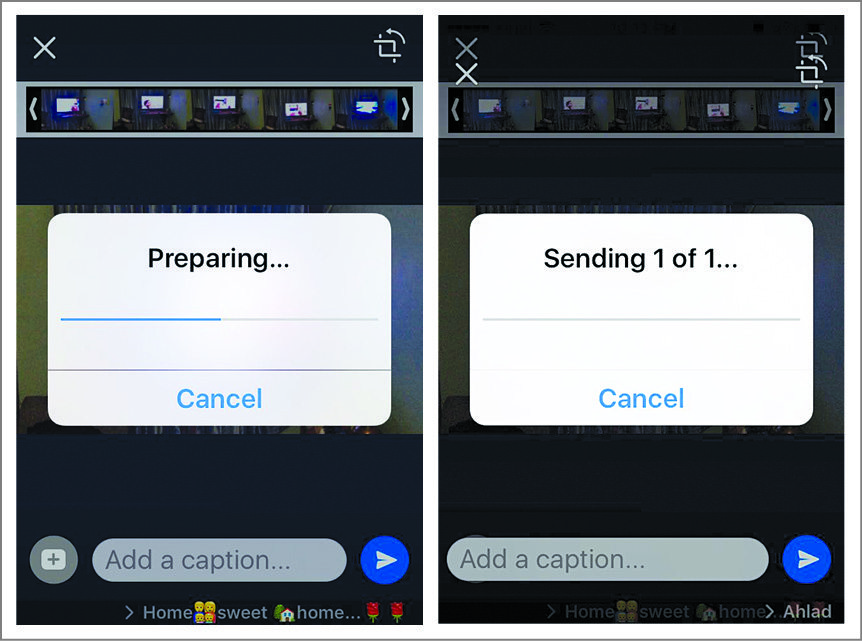
The main job of the image/video compression algorithm is to reduce the size of the file to be transmitted. For example, in the case of a 5MB video file, the image/video compression software running behind the preparing mode in WhatsApp software makes the video smaller by up to 1MB, thus saving the memory space for transmission to take place. The software performs this process automatically as you send the file to one of your friends. However, this process is visible only when the file to be transmitted is large in size, such as the 5MB video in this example.

Image compression is the task of representing an image with minimum number of coefficients so that the total memory occupied by the compressed image is much less than the original image. With this reduction of memory requirement for high-definition image, the transmission of these images onto the transmitting medium is much easier than without compression.

- Advertisement -

In order to achieve the task of image compression, it has to be represented in a domain where high-definition images/videos are sparse. The two existing domains widely used in digital signal processing are spatial domain and frequency domain.

The third domain widely used nowadays in the field of image processing is sparse domain. In this domain, mostly the coefficients are sparse in nature, i.e., most of them are zero with very few non-zero coefficients. Typically used techniques for transforming the spatial domain to sparse domain include wavelet, curvelet, singular value decomposition (SVD) and discrete cosine transform (DCT).

The concept of sparse domain is illustrated in Fig. 2 in a simple way. Fig. 2(a) shows a high-definition original image that occupies 2.3MB of space.

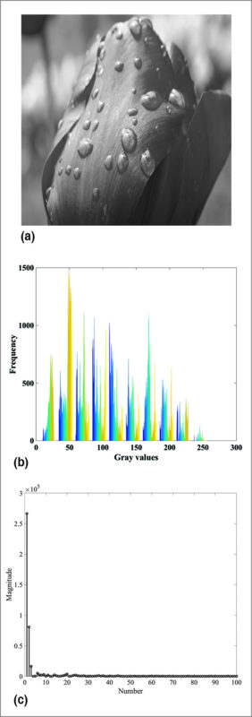
In spatial domain, this image is represented as a matrix of numbers, which are basically image-intensity levels. The plot of intensity levels, known as histogram of the image, is shown in Fig. 2(b). It can be observed from Fig. 2(b) that these intensity levels vary across a large range from 0 to 255. However, if you transform the same image using wavelet, curvelet, DCT or SVD domain, you get the plot of respective coefficients as shown in Fig. 2(c).

It can be observed that the same image can be represented using fewer coefficients as most of the coefficients in these domains are nearly zero. Hence, discarding these nearly-zero coefficients and retaining only non-zero coefficients reduces the memory space required to store these coefficients, which, in turn, helps in compressing the image.

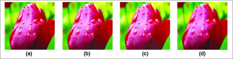
Here, we use DCT for image compression. Please note, it is not known what algorithm WhatsApp software is utilising for compressing its images and videos. Our intention in this article is to present the underlying concept behind the operation discussed in Fig. 1. Figure 3(a) shows a flower image that occupies 2.3MB of storage space. Using the DCT-based image compression algorithm, we obtained compressed images of sizes 392kB, 274kB and 223kB as shown in Figs 3(b)-(d), respectively. It can be seen, as the size of an image is compressed, artifacts tend to occur near the edges of the image. This is clearly visible in Fig. 3(d) where significant artifacts are visible.

The compression ratio is defined as:

K=Uncompressed size of an image/Compressed size of an image

For the images in Figs. 3(b)-(d), the value of K is obtained as 5, 8 and 10, respectively.
It can be observed from Fig. 3 that the images obtained after compression occupied less space and yet were good enough for visual inspection. Similar analysis is performed on grayscale image of a cameraman and the results are shown in Fig. 4.

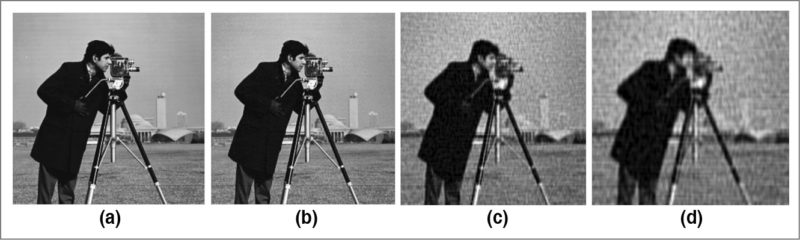
Here, the compression ratios for the images shown in Figs 4(b)-(d) are given as 5, 6 and 7, respectively. It can be seen, as the compression ratio increases from left to right, the blocking artifacts tend to appear in an image. This can be clearly seen from Fig. 4(d).

Testing procedure

The program (code.m) can be used for colour and grayscale images both. Tulip.jpeg colour image and cameraman.jpeg grayscale images were used during the testing of this program. You need to select one image (either colour or grayscale) at a time.

1. Install MATLAB R2013a or later version in your system. Open the code.m file

2. If colour image is to be compressed, line number 11 of the code.m file has to be uncommented. It is already uncommented for the given program

3. If grayscale image is to be compressed, line number 14 of the code.m file has to be uncommented.

4. Once you have selected either step 2 or step 3, select Run command button. Then the program prompts you to enter the threshold value. After entering this value followed by pressing Enter key, you need to wait for some time till the compressed image pops up on the screen.

5. For a coloured image, choose any one threshold value (e.g., 5, 50 or 500) for generating images shown in Figs 3(b)-(d), respectively.

6. For grayscale images, choose one threshold value (e.g., 10, 60 or 100) for generating images shown in Figs 4(b)-(d), respectively.

Download source code

This project was first published on 5 October 2017 and was updated on 26 March 2020.