Read Part 3
Image pre-processing and identification of certain shaped objects in the image is explained here using Image Deblurring and Hough Transform.
Image deblurring removes distortion from a blurry image using knowledge of the point spread function (PSF). Image deblurring algorithms in Image Processing Toolbox include Wiener, and regularised filter deconvolution, blind, Lucy-Richardson, as well as conversions between point spread and optical transfer functions. These functions help correct blurring caused by out-of-focus optics, camera or subject movement during image capture, atmospheric conditions, short exposure time and other factors.
deconvwnr function deblurs the image using Wiener filter, while deconvreg function deblurs with a regularised filter. deconvlucy function implements an accelerated, damped Lucy-Richardson algorithm and deconvblind function implements the blind deconvolution algorithm, which performs deblurring without the knowledge of PSF. We discuss here how to deblur an image using Wiener and regularised filters.
Deblurring using Wiener filter
Wiener deconvolution can be used effectively when frequency characteristics of the image and additive noise are known to some extent. In the absence of noise, Wiener filter reduces to an ideal inverse filter.
deconvwnr function deconvolves image I using Wiener filter algorithm, returning deblurred image J as follows:

J = deconvwnr(I,PSF,NSR)
where image I can be an N-dimensional array, PSF the point-spread function with which image I was convolved, and NSR the noise-to-signal power ratio of the additive noise. NSR can be a scalar or a spectral-domain array of the same size as image I. NSR=0 is equivalent to creating an ideal inverse filter.
Image I can be of class uint8, uint16, int16, single or double. Other inputs have to be of class double. Image J has the same class as image I.
The following steps are taken to read ‘Image_2.tif’, blur it, add noise to it and then restore the image using Wiener filter.
1. The syntax to read image (Image_2.tif) into the MATLAB workspace and display it is:
>> I=im2double(imread(‘Image_2.tif’));
>>imshow(I)
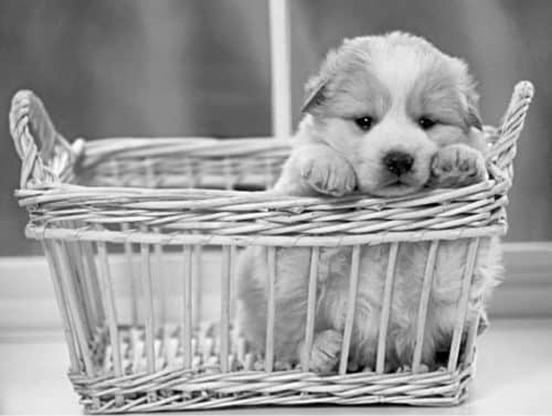
Fig. 1 shows the image generated by imshow function.
2. h=fspecial(‘motion’, len, theta) returns a filter to approximate the linear motion of a camera by len pixels, with an angle of theta degrees in a counter-clockwise direction. The filter becomes a vector for horizontal and vertical motions. The default value of len is 9 and that of theta is 0, which corresponds to a horizontal motion of nine pixels. B=imfilter(A,h) filters multidimensional array A with multidimensional filter h. Array A can be logical or non-sparse numeric array of any class and dimension. Result B has the same size and class as A. The syntax is:
>> LEN=21;
>> THETA=11;
>> PSF=fspecial(‘motion’,LEN,THETA);
>> blurred=imfilter(I,PSF,’conv’,’circular’);
>>figure,imshow(blurred)
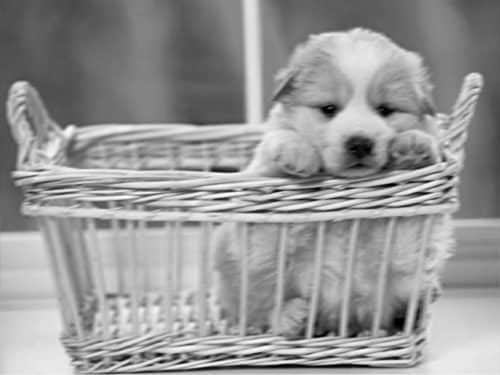
Fig. 2 shows the image generated by imshow function.
3. J=imnoise(I,’gaussian’,M,V) adds Gaussian white noise of mean M and variance V to image I:
>>noise_mean=0;
>>noise_var=0.002;
>>blurred_noise=imnoise(blurred,’gaussian’,
noise_mean,noise_var);
>>figure, imshow(blurred_noise)
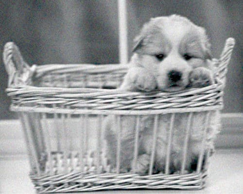
Fig. 3 shows the image generated by imshow function.
4. As mentioned above, J=deconvwnr (I,PSF,NSR) deconvolves image I using Wiener filter algorithm, returning deblurred image J. The following commands generate a deblurred image using NSR of zero:
>>estimated_nsr=0;
>> wnr2=deconvwnr(blurred_noise,PSF,
estimated_nsr);
>>figure,imshow(wnr2)

Fig. 4 shows the image generated by imshow function.
5. The following commands generate a deblurred image using NSR calculated from the image:
>>estimated_nsr=noise_var/var(I(:));
>> wnr3=deconvwnr(blurred_noise,PSF,
estimated_nsr);
>>figure,imshow(wnr3)
Fig. 5 shows the restored image from the blurred and noisy image using estimated NSR generated from the image.
Deblurring with a regularised filter
A regularised filter can be used effectively when limited information is known about the additive noise.
J=deconvreg(I, PSF) deconvolves image I using regularised filter algorithm and returns deblurred image J. The assumption is that image I was created by convolving a true image with a point-spread function and possibly by adding noise. The algorithm is a constrained optimum in the sense of least square error between the estimated and true images under requirement of preserving image smoothness.
Image I can be an N-dimensional array.
Variations of deconvreg function are given below:
• J = deconvreg(I, PSF, NOISEPOWER)
where NOISEPOWER is the additive noise power. The default value is 0.
• J = deconvreg(I, PSF, NOISEPOWER, LRANGE)
where LRANGE is a vector specifying range where the search for the optimal solution is performed.
The algorithm finds an optimal Lagrange multiplier LAGRA within LRANGE range. If LRANGE is a scalar, the algorithm assumes that LAGRA is given and equal to LRANGE; the NP value is then ignored. The default range is between [1e-9 and 1e9].
• J = deconvreg(I, PSF, NOISEPOWER, LRANGE, REGOP)
where REGOP is the regularisation operator to constrain deconvolution. The default regularisation operator is Laplacian operator, to retain the image smoothness. REGOP array dimensions must not exceed image dimensions; any non-singleton dimensions must correspond to the non-singleton dimensions of PSF.
[J, LAGRA] = deconvreg(I, PSF,…) outputs the value of Lagrange multiplier LAGRA in addition to the restored image J.
In a nutshell, there are optional arguments supported by deconvreg function. Using these arguments you can specify the noise power value, the range over which deconvreg should iterate as it converges on the optimal solution, and the regularisation operator to constrain the deconvolution.
Image I can be of class uint8, uint16, int16, single or double. Other inputs have to be of class double. Image J has the same class as Image I.
The following example simulates a blurred image by convolving a Gaussian filter PSF with an image (using imfilter):
1. Read an image in MATLAB:
>> I=imread(‘image_2.tif’);
>>figure,imshow(I)
Fig. 6 shows the image.
2. Create the PSF, blur the image and add noise to it:
>> PSF = fspecial(‘gaussian’,11,5);
>> Blurred = imfilter(I,PSF,’conv’);
>> V=0.03;
>>Blurred_Noise=imnoise(Blurred,
’gaussian’,0,V);
>>figure,imshow(Blurred_Noise)
Note that additive noise in the image is simulated by adding Gaussian noise of variance V to the blurred image (using imnoise). Fig. 7 shows the blurry and the noisy image.
3. The image is deblurred using deconvreg function, specifying the PSF used to create the blur and the noise power (NP):
>> NP=V*prod(size(I));
>> [reg1 LAGRA] = deconvreg(Blurred_
Noise,PSF,NP);
>>figure, imshow(reg1)
Fig. 8 shows the restored image.
Hough transform
The Hough transform is designed to identify lines and curves within an image. Using the Hough transform, you can find line segments and endpoints, measure angles, find circles based on size, and detect and measure circular objects in an image.
In the following Hough transform example we take an image, automatically detect circles or circular objects in it, and visualise the detected circles.
1. Read the image and display it. This example uses an image of circles of various colours:
>> I=imread(‘Image_3.png’);
>>figure, imshow(I)

Fig. 9 shows the image.
2. Determine radius range for searching circles. A quick way to find the appropriate radius range is to use the interactive tool imdistline, which gives an estimate of the radii of various objects.
h = imdistline creates a Distance tool on the current axis. The function returns h—handle to an imdistline object.
Distance tool is a draggable, resizable line, superimposed on an axis, which measures the distance between two endpoints of the line. It displays the distance in a text label superimposed over the line. The tool specifies the distance in data units determined by XData and YData properties, which is pixels by default.
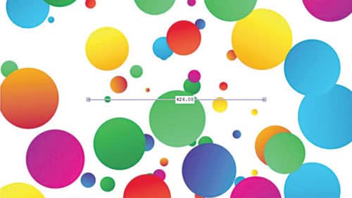
If you wrote the following command in MATLAB, Fig. 9 would change to that shown in Fig. 10:
>>d = imdistline
The line can be dragged to get the size of different circles.
In a nutshell, imdistline command creates a draggable tool that can be moved to fit across a circle and the numbers can be read to get an approximate estimate of its radius.
To remove the imdistline tool, use the function:
>>delete(d);
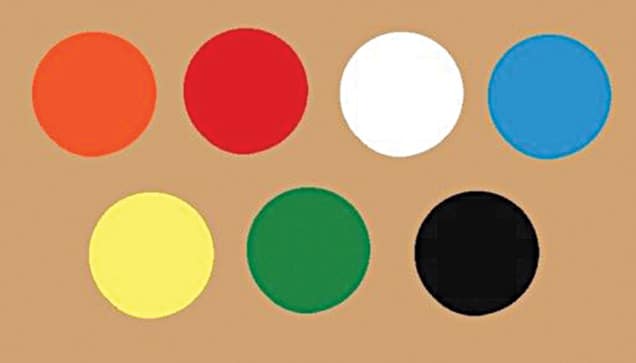
3. Consider the image shown in Fig. 11. The aim is to find the number of circles in the figure.
Quite evidently, there are many circles having different colours with different contrasts with respect to the background. Blue and red circles have strong contrast with respect to the background, whereas white and yellow circles have the poorest contrast with respect to the background.
4. We calculate the objects that are brighter and those that are darker than the background. For this, we need to convert this RGB image into grayscale version:
>> RGB=imread(‘Image_4.png’);
>>gray_image=rgb2gray(RGB);
>>figure, imshow(gray_image)
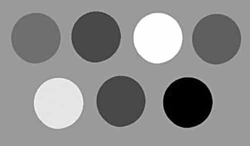
Figure 12 shows the grayscale image
5. Function centers=imfindcircles (A,radius) finds circles in image A whose radii are approximately equal to radius. The output, centers, is a two-column matrix containing (x, y) coordinates of centers of the circles in the image.
[centers,radii] = imfindcircles (A,radiusRange) finds circles with radii in the range specified by radiusRange. The additional output argument, radii, contains the estimated radii corresponding to the center of each circle in centers.
By default, imfindcircles finds circular objects that are brighter than the background. In our case, let us set the parameter ‘ObjectPolarity’ to ‘dark’ in imfindcircles to search for dark circles:
>> [centers,radii]=imfindcircles(RGB,
[40 60],’ObjectPolarity’,’Dark’)
The result of the above command is:
centers = 384.2814 204.1827
radii = 50.1646
As you can see, only one circle is detected. This happens because imfindcircles is a circle detector, and similar to most detectors, imfindcircles has an internal detection threshold that determines its sensitivity. imfindcircles has a parameter ‘sensitivity’ that can be used to control this internal threshold, and consequently, the sensitivity of the algorithm. A higher sensitivity value sets a lower detection threshold and leads to detection of more circles. This is similar to the sensitivity control on motion detectors used in home security systems.
6. By default, sensitivity, which is a number between 0 and 1, is set to 0.85. Increase sensitivity to 0.9:
>> [centers,radii]=imfindcircles(RGB,
[40 60],’ObjectPolarity’,’Dark’,
’Sensitivity’,0.9)
You will get:
centers =
384.2002 204.0138
248.6127 201.3416
198.2825 73.5618
442.8091 77.9060
radii =
50.1646
50.2572
50.2951
49.7827
By increasing sensitivity to 0.9, the function imfindcircles found four circles. ‘centers’ contains center locations of circles and ‘radii’ contains the estimated radii of these circles.
7. Function viscircles can be used to draw circles on the image. Output variables ‘centers’ and ‘radii’ from function imfindcircles can be passed directly to function viscircles:
>>imshow(RGB)
>> h=viscircles(centers,radii)

Fig. 13 shows the result.
As you can see from Fig. 13, centers of circles seem to be correctly positioned and their corresponding radii seem to match well to the actual circles. However, quite a few circles were still missed. Let us increase ‘Sensitivity’ to 0.928:
>> [centers,radii]=imfindcircles(RGB,
[40 60],’ObjectPolarity’,’Dark’,
’Sensitivity’,0.98)
centers =
384.2193 204.4776
248.8446 201.4930
197.7027 73.5149
442.9998 78.3674
76.7218 76.5162
radii =
50.1646
50.2572
50.2951
49.7827
50.4039
Now, we are able to detect five circles. Hence, by increasing the value of sensitivity you can detect more circles. Let us plot these circles on the image again:
>>delete(h); % Delete previously drawn
circles
>>h = viscircles(centers,radii);

Fig. 14 shows the result.
8. As you can see, function imfindcircles does not find yellow and white circles in the image. Yellow and white circles are lighter than the background. In fact, these seem to have very similar intensities as the background. To confirm this, let us see the grayscale version of the original image again. Fig. 15 shows the grayscale image.
>>figure, imshow(gray_image)
9. To detect objects brighter than the background, change ‘ObjectPolarity’ to ‘bright’:
>> [centers,radii]=imfindcircles(RGB,
[40 60],’ObjectPolarity’,’Bright’,
’Sensitivity’,0.98)
centers =
323.2806 75.9644
122.3421 205.1504
radii =
49.7654
50.1574
10. Draw bright circles in a different colour by changing ‘Colour’ parameter in viscircles:
>>imshow(RGB)
>>hBright=viscircles(centers,radii,
’Color’,’b’);
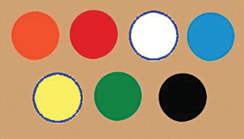
Fig. 16 shows the image.
11. There is another parameter in function imfindcircles, namely, EdgeThreshold, which controls how high the gradient value at a pixel has to be before it is considered an edge pixel and included in computation. A high value (closer to 1) for this parameter will allow only the strong edges (higher gradient values) to be included, whereas a low value (closer to 0) is more permissive and includes even the weaker edges (lower gradient values) in computation. Therefore, lower the value of EdgeThreshold parameter, more are the chances of a circle’s detection. However, it also increases the likelihood of detecting false circles. Hence, there is a trade-off between the number of true circles that can be found (detection rate) and the number of false circles that are found with them (false alarm rate).
Following commands detect both the bright and the dark objects and encircle them:
>>[centersBright,radiiBright,metricBright]
=imfindcircles(RGB,[4060], ‘ObjectPolarity’,
’bright’,’Sensitivity’,0.9,’EdgeThreshold’,
0.2);
>>imshow(RGB);
>> h=viscircles(centers,radii);
>>hBright=viscircles(centersBright,
radiiBright,’Color’,’b’);
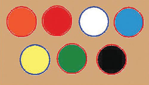
Fig. 17 shows the output image.
For reading other MATLAB projects: click here