
Scalability. It should be scalable in terms of the computer memory. If it consumes a large memory then surely it would be unacceptable.
Flexibility. Generally, one method produces best result for one type of problem. The implementation should be made flexible so that it would produce stable results for other type of problems as well.
Parallelisation. For fast results, one computer is not enough. So it must offer parallel computing.

The computing cost depends on size of the solution and time required to find the solution. It should be as low as possible. At the core of computational electromagnetics is the numerical method used for a specific problem. Broadly, there are two types of methods for solving EM problems:
Analytical method. This gives an insight into the process but is generally limited to idealised processes only.
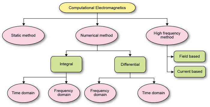
Numerical method. This gives an approximate solution of any type of problem and structure. With numerical method the analysis and prototyping of complex systems is easy. It also allows investigation of material properties without performing any experiment, besides easy optimisation and modification for its implementation. Presently, simulators use a combination of both the methods to reduce the computational cost.
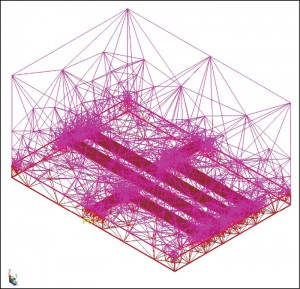
Implementation of CEM (Fig. 2) efficiently is not an easy task. There are various problems associated with their implementation, such as the type of material to be analysed (homogeneous/inhomogeneous, isotropic/anisotropic, etc), type of geometry (regular/irregular, large/small, etc), undetermined problems like those when there are resonating structures within the geometry or when the material contradicts in the problem.
Many advanced concepts, such as iterative solvers, preconditioned algorithms, domain decomposition methods and parallel computing, have been developed and implemented in present solvers.
CEM implementation has several disadvantages with the major one being the theoretical model results. The process is purely theoretical with no resemblance to experiments. So it would definitely need a validation with the practical results. Second, there will be numerical method error and mesh error that would go unnoticed, if not validated.
Numerical methods
The Maxwell equation can be written in two forms: integral and differential. Literally, integration means joining things and differentiation means dividing them. This literal definition of the two basically helps in determining which type of geometry can be applied with which type of Maxwell equation. If the geometry is planar and complex then the numerical method using integral Maxwell equation would be preferred.
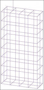
The material boundaries in complex geometry cause discontinuities in the electric and magnetic fields. The type of Maxwell equations are then applied to these discontinuities, thus reducing the problem to algebraic expression (integral ones) and difference expressions (in case of differential Maxwell equation). Numerical methods employing differential Maxwell equation discretise the geometry by volumetric mesh (hexahedrons and tetrahedrons) and require an extra absorption boundary condition (ABC) type boundary over the geometry. In these methods the computations are done for the EM fields.
The numerical methods employing integral form of Maxwell equation discretise the geometry by surface mesh (triangular, quads) and do not require extra boundary over the geometry. Computations are done for the current and charge although the 3D patterns can be generated.
What determines the choice of numerical method
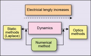
Apart from the planar and 3D type geometry the numerical method is chosen on the basis of required accuracy of the result, the memory limitation of method, what different type of material properties it can handle, whether the results have to be in time domain or in frequency domain, what would be its operating frequency, etc. These are secondary factors. The primary factor that determines the type of numerical method is the electrical size/length of the structure itself.
Electrical length is defined as ratio of physical length of device to the operating wavelength. As the electrical length increases or decreases, method to be used will also vary, as shown in Fig. 4.