
Domains in which solvers works
Like time and frequency domains in the signal analysis, the CEM techniques are also domain-specific and are optimised for those. For CEMs there are basically five domains, namely, static, time, frequency, Eigen and ray tracing, as depicted in Fig. 5.
Static. In this domain there is no time variation of the equations and it is mostly used for DC bias field configuration of low field approximation.
Time. In this method the unknown field quantities are real-time varying in nature. This method does not use traditional matrix method, instead nearest neighbour interaction is calculated and interpolated. The applied source is impulsive in nature.

Frequency. This is a good choice if we need to calculate results all over the bandwidth of the centre frequency. The excitation is sinusoidal in nature and broadband results are transformed into time domain by inverse Fourier transform. However, for low frequency this method is unsuitable, so in that case we need to use static domain methods. Also, each frequency needs separate computation, so frequency sweep should be selected appropriately. Otherwise, it would take a lot of memory.
Eigen. In this domain no excitation source is applied. This method is used to find the resonant frequencies and propagation modes of the waveguide, cavity, propagation constant, etc. The results are field configurations that would be preferred to be excited by real environmental sources.
Ray tracing (or optics). As the electrical size increases, the integral and differential methods become useless. Then the optics method combines the Green’s function to calculate fields by current and then uses the boundary conditions to determine current induced on the objects. This domain has two methods: PO and UTD.
Methods using integral Maxwell equations
Method of moments (MOM). Also known as 3D planar method, it uses Green’s function over the planar structure, thus reducing the Maxwell equations to algebraic expressions. Layered stack up-structures can also be analysed as the Green’s function can be applied, thus x-y plot is established as in planar structure. It actually approximates the current distribution as sum of basic functions. In this method the calculations are required only at boundary values and not throughout the space, as shown in Fig. 6.
MOM creates a surface mesh over the modelled surface. MOM solutions are typically limited to objects that are only one or two wavelengths in size, for example, to calculate and extract detailed multiport s-parameter of all the interconnects on PCBs. Analysis of large structures becomes difficult because of the large amount of memory and time required to compute.
Some disadvantages of the MOM method are:
1. As the geometry increases, the storage requirement and computing time increase as the square of the size of geometry.
2. It can be applied only to those problems for which the Green’s function can be calculated.
3. Different frequencies require different formulations (due to frequency domain).
4. It does not satisfy boundary condition at every point; satisfies only over an integral average of boundaries.
Multilevel fast multipole method (MLFMM). It is an alternative approach to the MOM as it requires less memory. It is suitable for analysis of very large problems, such as RCS and reflector antenna. According to emfieldsolution.com, “The object is placed in a box which is then split into eight smaller boxes. Each of the boxes is then divided again recursively until the size of smaller boxes contains few basic functions.” It also illustrates that, if a particular MOM solution requires 150GB memory then MLFMM would require only 1GB.
Partial element equivalent circuit (PEEC). In this method the integral equations are interpreted as Kirchhoff’s voltage law applied to basic cell. So, overall, the geometry in this method would result in a complete circuit, and it also allows some circuit elements to be added easily—an edge over the other solvers. This type of solver allows analysis both in time and frequency domain.
Methods using the differential Maxwell equations
Finite-difference time domain (FDTD). It is a time domain technique and thus a single simulation can cover a wide frequency range. This method allows easy computations for each cell made of different materials. After the process, the time domain results are converted to frequency domain by the use of DFT techniques.
Consider a large structure. This method will not produce dense material matrices (as done by others); it will include only the nearest neighbour interaction. This method can cover frequencies from near low to microwave, and up to visible light frequencies. The discretisation grid used is rectangular (usually) and separate grids are used for E and H calculations.
A disadvantage of the method is that, although one simulation will work for a wide frequency range, this is not the case with the ports. A single simulation has to run for each port placed on the geometry. So, if there are N ports in a structure, N simulations would be required.
Some applications of the method are:
1. Time domain reflectrometry (TDR)
2. Antenna placement on cars, trains, etc
3. Simulation of phone with SAM head to calculate SAR value
4. When the module is electrically large and ports are less
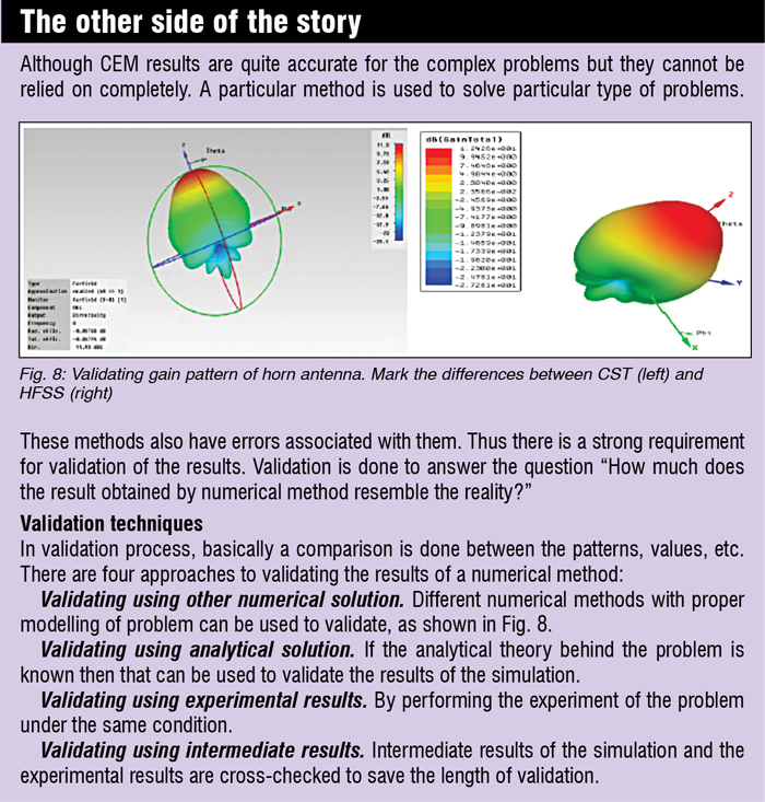
Finite element method (FEM). It is defined as an approximation technique to discretise geometric objects. Each part of discretised structure is called a finite element. It is a frequency-domain flexible method for geometrical and material handling of closed structures. It generates a sparse matrix of unknown field quantities. This method requires meshing of entire space and needs additional ABC boundary over the structure to be analysed. The unknown field quantities are approximated over each mesh as sum of functions, as shown in Fig. 8.
Its disadvantage is that, for simulation of structures of complex and electrically large geometries, the mesh may become very complex. And that would result in large matrices which would require huge memory resources.
Its advantages are:
1. It is most suitable for high ‘Q’ circuits
2. Useful for analysis of filters, cavities, resonators, etc
3. Provides good results for geometries with large number of ports, such as IC packages and multi-chip modules.
Apart from these, several other methods like FIT (finite integration method) over FEM, TLM over FDTD, MLFMM over MOM have been developed, but their basic functioning is based on the methods described above.
High frequency methods
For computing field quantities of Maxwell equation at electrically large structures, optical methods have been developed. These methods can be divided into (a) field -based methods like UTD (uniform theory of diffraction) and (b) current-based methods like PO (physical optics).
In PO method the current distribution is calculated by the use of Green’s function (MOM) and then this distribution is applied to the boundary conditions of the structure. Then calculations are performed on the structure by inducing that current distribution and updating the main results. The incident wave on the structure continues or passes through it as if the structure was not present.
The UTD method employs a different strategy. Here also the current distribution is applied to the boundary condition but the structure blocks the incident waves on each part of the structure. The field quantities are then determined from the diffracted waves. Consider a reflector antenna with excitation as a dipole antenna placed in front of it. The pattern and quantities will be calculated by PO in the front region while the backside region will be computed by UTD.
CST, HSS, FEKO solver overview
Computer simulation technology microwave studio (CST MWS) is one of the most comprehensive tools for RF designers and engineers. It provides the maximum of six solvers, namely:
1. Time domain solver. It uses hexahedral mesh and is very efficient for high frequencies. It provides two alternative methods: transient solver (FIT) and TLM solver (for better simulation of EMC/EMI models). It calculates transmission of energy between various ports and open structures of the model. Typical applications include TDR, RCS and dispersive materials.
2. Frequency domain solver. It uses hexahedral and tetrahedral mesh.
3. Eigen mode solver. It is recommended strongly for loss-free structures.
4. Integral solver. It uses MLFMM technique.
5. Multilayer solver. For planar structures as it is based on MOM.
6. Asymptotic solver. It uses optical techniques for electrically large structures.
Apart from CST, HFSS and FEKO are also widely used softwares for CEM applications. HFSS provides two solvers: FEM and HFSS-IE (MLFMM based). FEKO provides five solvers: FEM, MOM, PO, UTD and MLFMM.
The author, a B.Tech in EC, has contributed some other interesting articles as well in the past